In this short post, I want to define Shared Risk Link Groups and illustrate this with an interactive plot using Grave and Networkx.

Shared Risk Groups

Shared Risk (Resource) Group is an important concept in Network Theory. This concept may arise in different types of networks (IP, optical, MPLS). Generally, there are two networks to be considered: physical and virtual. A set of pre-computed paths in physical is in one-to-one correspondence with links of the virtual graph. If a single physical edge is broken, some subset of virtual edges also fails; this subset is called a Shared Risk Link Group.

Example from Optical Networks

A typical example I have personally worked with is Shared Risk Link Groups in optical mesh networks. Edges in optical networks correspond to fibers and paths in optical networks are called optical channels. Assume that there is a set of established optical channels; a service provider wants to satisfy network demands and route them using established optical channels.

Usually, every demand requires two (or more) paths called working and protection; if the working path fails, the protection path ensures non-disrupted information delivery. However, there is a difficult condition to be satisfied: if a single optical edge fails (and thus some set of optical channels fails), at least one of the working/protection paths should stay online for every demand.

Interactive Networkx

We will need the following imports and have Grave library installed.

import networkx as nx
import numpy as np
import matplotlib.pyplot as plt
from grave import plot_network
from grave.style import use_attributes
import itertools
import random

First, we prepare some data for visualization and generate a toy optical network:

random.seed(a = 17)

graph = nx.compose(nx.cycle_graph(20), nx.random_tree(10))
pos = nx.kamada_kawai_layout(graph)
shift = 3.0

def lex(edge):
    return tuple(sorted(list(edge)))

service_num = 15
endnodes = list(itertools.combinations(graph.nodes(), 2))
endnodes = random.sample(endnodes, k = service_num)
srlg = {}
for edge in graph.edges():
    srlg[lex(edge)] = set([])

Now we generate optical channels and links of a virtual graph:

for st in endnodes:
    path = nx.shortest_path(graph, source=st[0], target=st[1])
 
    Vst = ("V"+str(st[0]), "V"+str(st[1])) 
    graph.add_edge(*Vst)
    pos[Vst[0]] = np.array([pos[st[0]][0], pos[st[0]][1] + shift])
    pos[Vst[1]] = np.array([pos[st[1]][0], pos[st[1]][1] + shift])
    
    srlg[lex(Vst)] = set([Vst])
    edges = [(path[i], path[i+1]) for i in range(len(path) - 1)]
    for edge in edges:
        srlg[lex(edge)].add(Vst)

The hilighter function is a minor update from example:

def hilighter(event):
    # if we did not hit a node, bail
    if not hasattr(event, 'edges') or not event.edges:
        return

    # pull out the graph,
    graph = event.artist.graph

    # clear any non-default color on edges

    for u, v, attributes in graph.edges.data():
        attributes.pop('color', None)

    for edge in event.edges:
        graph.edges[edge]['color'] = 'red'
        for failed_edge in srlg[lex(edge)]:
            graph.edges[failed_edge]['color'] = 'red'
    
    # update the screen
    event.artist.stale = True
    event.artist.figure.canvas.draw_idle()

The decorator below is a solution that allows passing my precomputed layout into the plot_network function.

def make_layout(pos):
    def layout(graph):
        return pos
    return layout

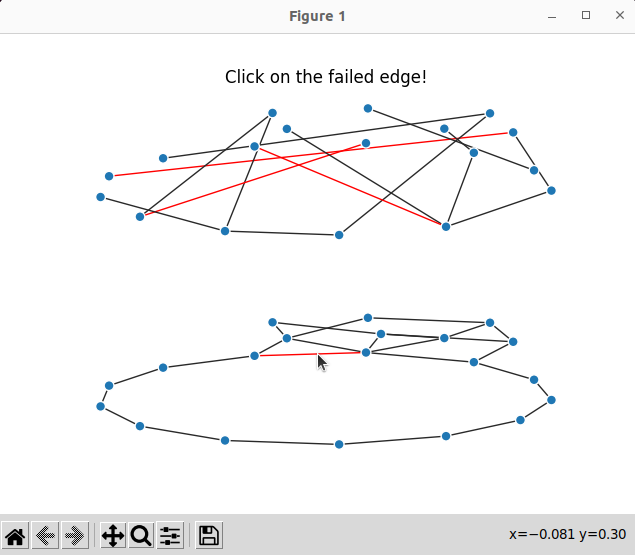
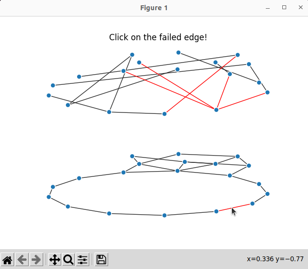
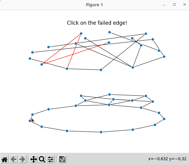
Result

Now we can run the code below

fig, ax = plt.subplots()
art = plot_network(graph, layout=make_layout(pos), ax=ax, node_style=use_attributes(),
                   edge_style=use_attributes())

art.set_picker(10)
ax.set_title('Click on the failed edge!')
fig.canvas.mpl_connect('pick_event', hilighter)
plt.show()

which produce interactive plots; here we can click on an optical edge and see which optical channels fail: